Section author: Sebastian Jentschke, Rebecca Vederhus

From SPSS to jamovi: Logistic Regression

This comparison shows how a binary logistic regression is conducted in SPSS and jamovi. The SPSS test follows the description in chapter 20.5 - 20.6 in Field (2017), especially figure 20.7 - 20.10 and output 20.1 - 20.5 (bootstrap excluded). It uses the data file Eel.sav which can be downloaded from the web page accompanying the book.

SPSS	jamovi
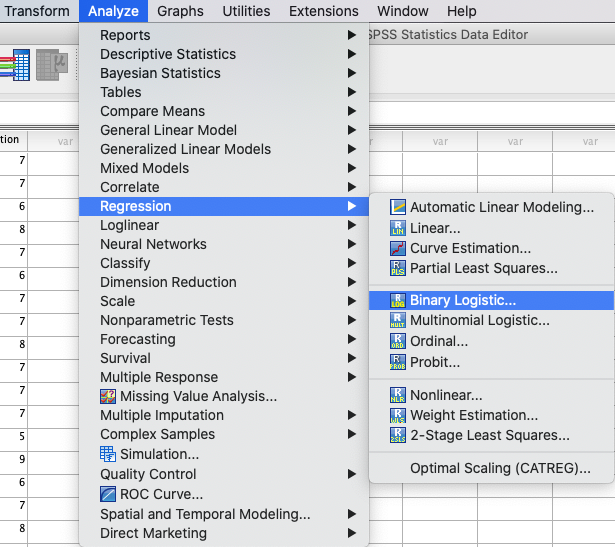
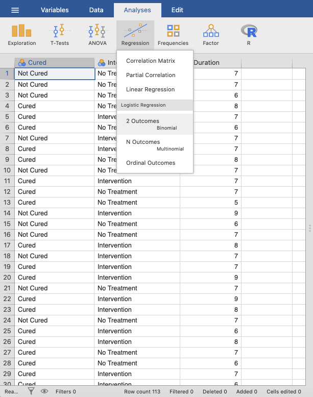
In SPSS you can run a binary logistic regression using: Analyze → Regression → Binary Logistic.	In jamovi you do this using: Analyses → Regression → 2 Outcomes Binominal.
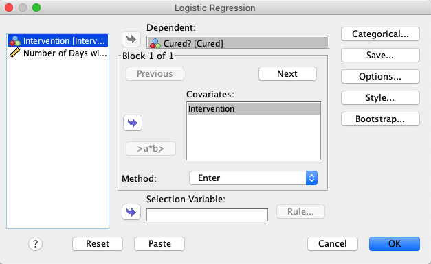
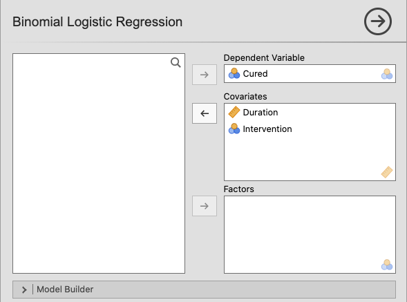
In SPSS, move Cured to the Dependent variable box and Intervention to the Covariates variable box.	In jamovi, move the variable Cured to Dependent Variable and the variables Duration and Intervention to Covariates.
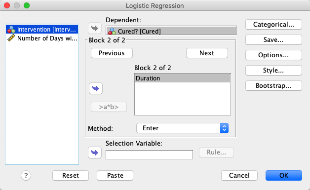
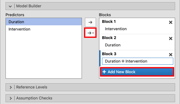
Click Next and add Duration to this new block.	Create two new blocks by clicking + Add New Block in the Model Builder drop-down menu. Add the Duration variable to Block 2, and add Duration and Intervention to Block 3 by marking them both and clicking Interaction in the drop-down menu.
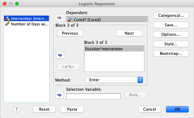
Create a third block by clicking Next one more time, and create an interaction by marking both Intervention and Duration and moving them to the block by pressing the arrow.
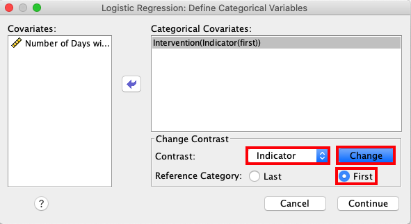
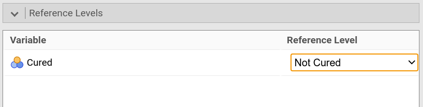
Access the Categorical window and open the drop-down menu for Contrast. Here, choose Indicator and then check First as the Reference Category. Click Change.	jamovi set the reference category automatically to the first category. If you were to change that, open the drop-down menu Reference levels, and change the reference level for each variable to the desired level (e.g., Not Cured).
Open the Options window and check the following boxes: Classification plots, Hosmer-Lemeshow goodness-of-fit, Casewise listing of residuals, Outliers outside 2 std. dev., Iteration history, CI for exp(B), At each step, and Include constant in model.	Open the drop-down menu Prediction and tick Classification table.
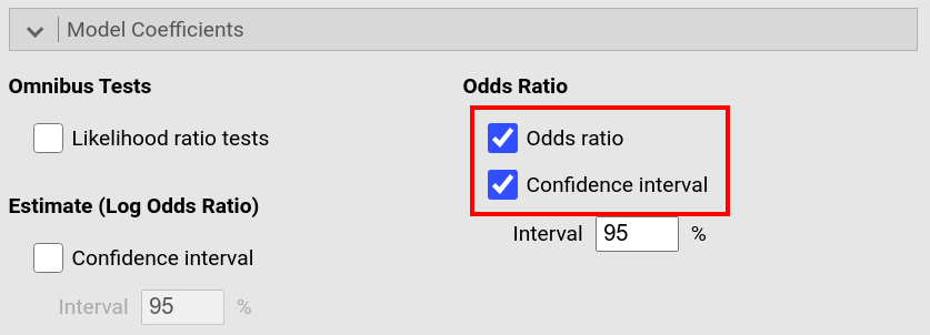
	In the drop-down menu Model Coefficients, tick Odds ratio and the Confidence interval to odds ratio.
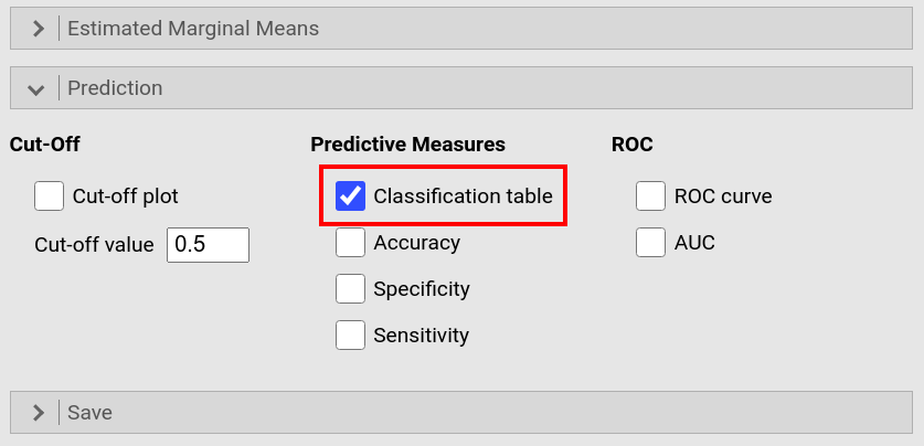
	In the Model Fit window, check the boxes for Deviance, AIC, Overall Model Test, Cox & Snell's R² and Nagelkerke's R².
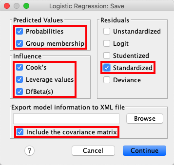
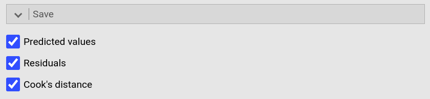
Open the Save window and check Probabilities, Group membership, Cook's, Leverage values, DfBeta(s), Standardized (residuals), and Include the covariance matrix.	jamovi permits you to save some of these values too. To do so, open the drop-down menu Save and tick Predicted values, Residuals, and Cooks's distance.
If you compare the output from SPSS and jamovi, the results are essentially the same. However, the results from jamovi are shorter and better structured, whereas the SPSS results are much more extensive (likely to the more comprehensive choice of options, according to Field, 2017). jamovi, furthermore, first has an overview over the models and their comparison whereas SPSS provides those model indices within each model.
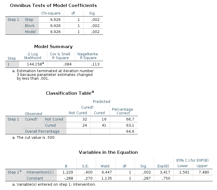
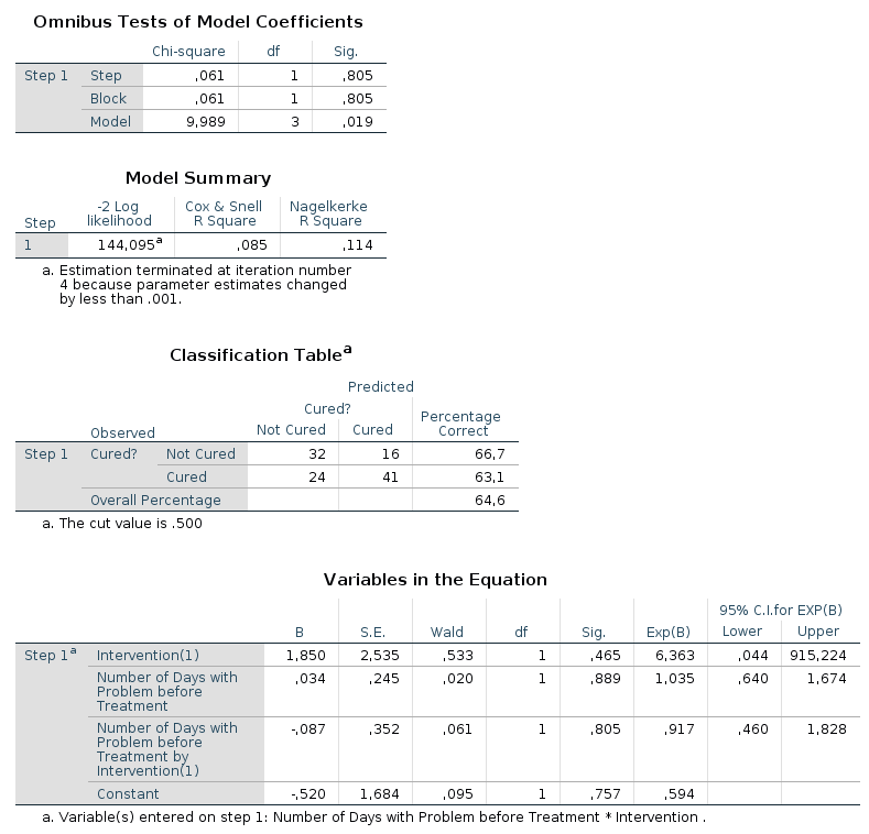
In the output from SPSS you can find tables for Model Summary, Variables in the Equation and Omnibus Tests of Model Coefficients for each of the predictors in the model. The Model Summary tables shows the -2LL value for the model, as well as Cox & Snell R² and Nagelkerke R². In the Omnibus Tests of Model Coefficients tables, χ²-values, degrees of freedom and significance values are found. Lastly, you can find b-values, SE-values, degrees of freedom and significance values in the Variables in the Equation table. This table also shows the odds ratio.	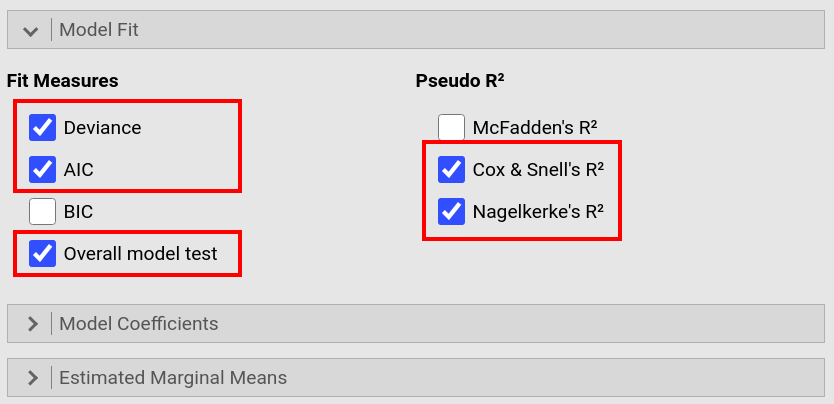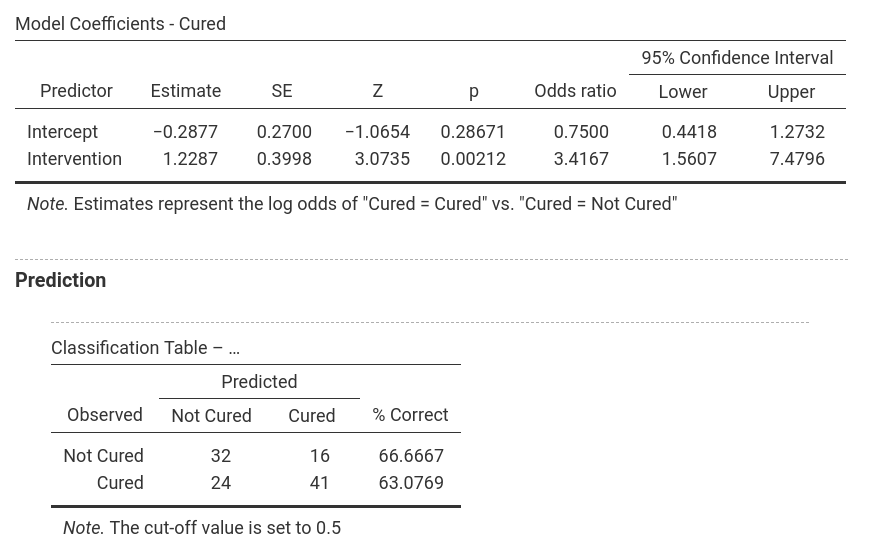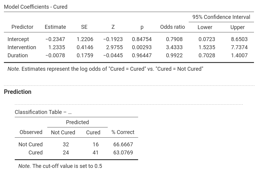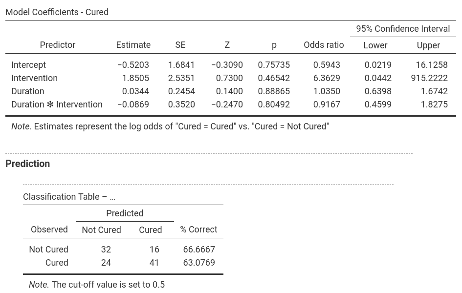In jamovi, -2LL values, Cox & Snell R² and Nagelkerke R² values for all the predictors are found in the table called Model Fit Measures. χ²-values, degrees of freedom and significance levels are found in the Model Comparisons table. In addition, b-values, SE-values, significance level odds ratio and the confidence interval for it as well as the classification table are shown as separate parts of the output (one for each model). Only one model is shown at a time and the model can be selected by using the drop-down menu next to Model Specific Results.
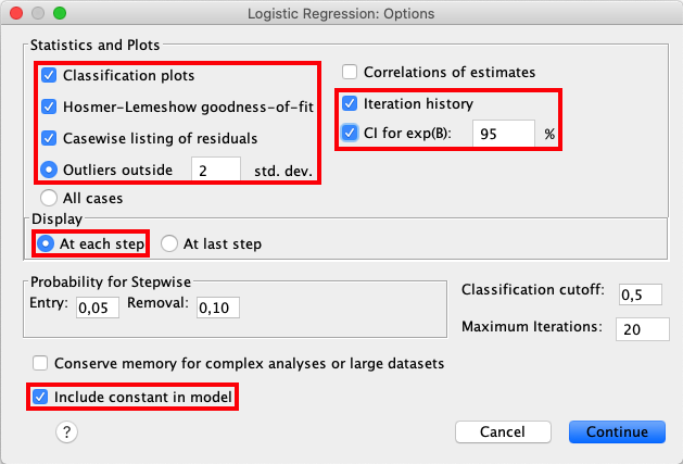
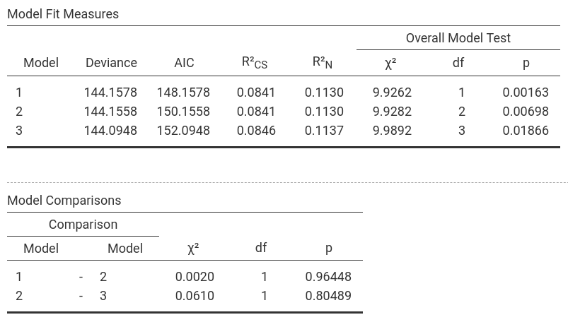
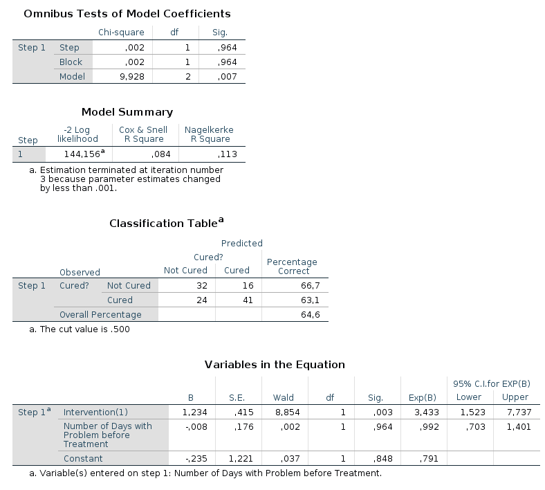
SPSS produces a lot more output tables (some not shown) than jamovi, not the least due to Field (2017) asking for options that are not available in jamovi. The numerical values for the results are the same. Model 1: -2LL = 144.158, χ² = 9.926, df = 1, p = 0.002, R²CS = 0.084, R²N = 0.113, corr.NC = 66.667, corr.C = 63.077 Model 2: -2LL = 144.156, χ² = 9.928, df = 2, p = 0.007, R²CS = 0.084, R²N = 0.113, corr.NC = 66.667, corr.C = 63.077 Model 3: -2LL = 144.095, χ² = 9.989, df = 3, p = 0.019, R²CS = 0.085, R²N = 0.114, corr.NC = 66.667, corr.C = 63.077 It becomes clear that Intervention is the most decisive predictor whereas Duration and the interaction of Intervention × Duration don’t really lead to better prediction: The number of correctly classified cases doesn’t change between the models while Model 1 is the most parsimonuous; furthermore, the Deviance (-2LL) and χ² for Model 2 and 3 are more or less the same as for Model 1 (and since more df’s are used in Model 2 and 3, the p-values increase (which is all emphasizing that Model 1 is the best model and should be selected).
If you wish to replicate those analyses using syntax, you can use the commands below (in jamovi, just copy to code below to Rj). Alternatively, you can download the SPSS output files and the jamovi files with the analyses from below the syntax.
LOGISTIC REGRESSION VARIABLES Cured /METHOD=ENTER Intervention /METHOD=ENTER Duration /METHOD=ENTER Duration * Intervention /CONTRAST (Intervention)=Indicator(1) /SAVE=PRED PGROUP COOK LEVER DFBETA ZRESID /CLASSPLOT /CASEWISE OUTLIER(2) /PRINT=GOODFIT ITER(1) CI(95) /CRITERIA=PIN(0.05) POUT(0.10) ITERATE(20) CUT(0.5).	jmv::logRegBin( data = data, dep = Cured, covs = vars(Duration, Intervention), blocks = list(list("Intervention"), list("Duration"), list(c("Duration", "Intervention"))), refLevels = list(list(var="Cured", ref="Not Cured")), pseudoR2 = c("r2mf", "r2cs", "r2n"))
SPSS output file containing the analyses	jamovi file containing the analyses

References

Field, A. (2017). Discovering statistics using IBM SPSS statistics (5th ed.). SAGE Publications. https://edge.sagepub.com/field5e