Section author: Laiton Hedley

Common Data Recipes

This section provides step-by-step recipes for the most common data handling tasks in jamovi.

Reverse Scoring Survey Items

When handling survey data, some items are reverse scored — higher scores on those items indicate less of the construct being measured. A simple rule of thumb: subtract the item score from the maximum possible score plus one.

For example, participants have responded on a 1–7 Likert scale to three items, but Item_3 is scored in the opposite direction:

Table 15 Data before reverse scoring

Item_1	Item_2	Item_3
4	3	3
3	4	5
4	4	2

Single item: create a computed variable with a direct formula.

1. Click a new column and choose New Computed Variable.

2. Enter the formula: 8 - Item_3

Multiple items (same formula): use a transformed variable so you can apply the same formula to several columns at once.

1. Click a new column and choose New Transformed Variable.

2. Select the item as the source variable.

3. Click Using transformation and choose Create New Transform….

4. Enter the formula: 8 - $source

Table 16 Data after reverse scoring Item_3

Item_1	Item_2	Item_3	Item_3_Reversed
4	3	3	5
3	4	5	3
4	4	2	6

Higher scores on Item_3_Reversed now indicate more of the construct, consistent with Item_1 and Item_2. This step is important before computing a sum or mean score across items.

Summation (or Total) Score of Survey Items

Sum scores combine multiple survey items into a single overall score for a construct — for example, to measure a personality trait such as Extraversion (more info).

Below are responses to four items of an Extraversion subscale, each scored on a 1–5 Likert scale:

Table 17 Data before computing sum score

Item_1	Item_6	Item_11	Item_16
5	1	3	3
4	2	1	1
4	2	4	5

1. Click a new column and choose New Computed Variable.

2. Use the SUM() function with all item names:

   SUM(Item_1, Item_6, Item_11, Item_16)

Table 18 Data after computing sum score

Item_1	Item_6	Item_11	Item_16	Extraversion_Sum_Score
5	1	3	3	12
4	2	1	1	8
4	2	4	5	15

The new column contains the overall score for each participant.

Recoding a Continuous Variable to Categories

Continuous variables are often recoded into categories for group comparisons. Age is a common example — it can be grouped into Young Adults (18–29), Middle-Aged Adults (30–59), and Older Adults (60+).

Table 19 Age data before recoding

Age
25
18
35
45
65

1. Click a new column and choose New Transformed Variable.

2. Select Age as the source variable.

3. Click Using transformation and choose Create New Transform….

   

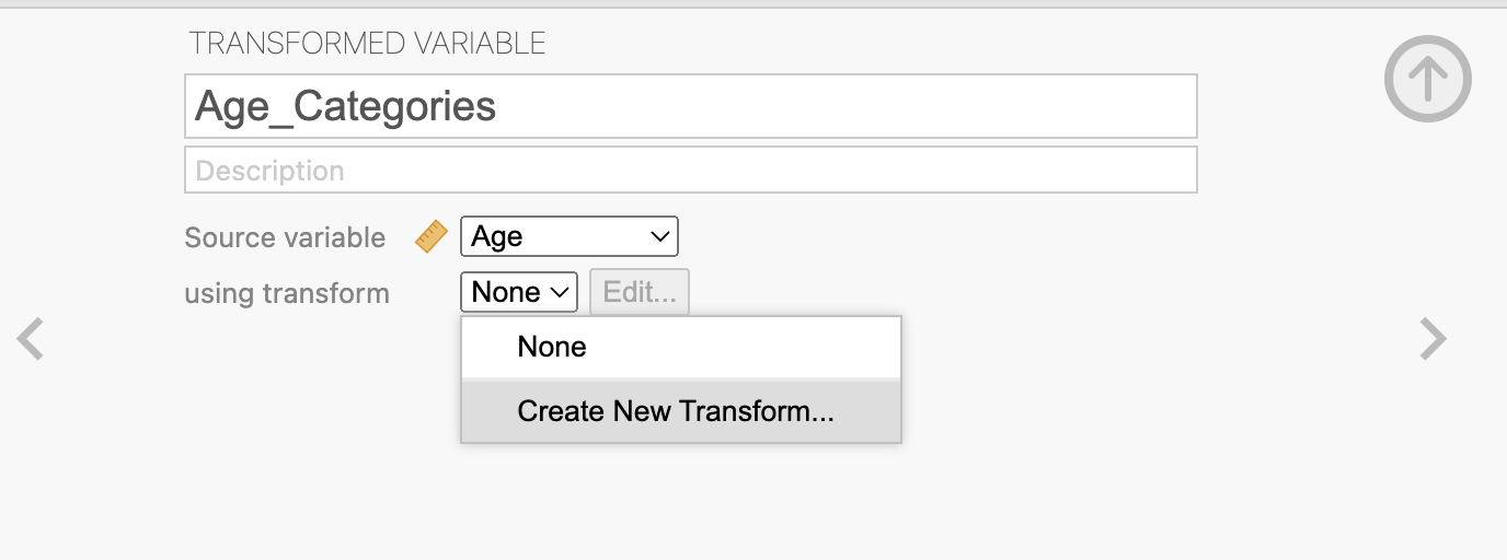
4. Click Add recode condition and set up the following conditions:

   

   • If $source < 30, assign 'Young'

   • If $source < 50, assign 'Middle-Aged'

   • Else, assign 'Older'

   Conditions are evaluated in order, so values below 30 are assigned “Young” first, then values below 50 become “Middle-Aged”, and all remaining values become “Older”.

Table 20 Age data after recoding

Age	Age_Category
25	Young
18	Young
35	Middle-Aged
45	Middle-Aged
65	Older

Recoding/Reducing the Number of Categories

Categorical variables with many levels can be reduced to fewer categories for simpler analysis. For example, smoker status may have four levels (Non-smoker, Occasional Smoker, Regular Smoker, Heavy Smoker) that can be collapsed into two (Non-smoker, Smoker).

Table 21 Smoker status before recoding

Smoker_Status
Non-smoker
Occasional Smoker
Regular Smoker
Heavy Smoker

1. Click a new column and choose New Transformed Variable.

2. Select Smoker_Status as the source variable.

3. Click Using transformation and choose Create New Transform….

4. Set up recode conditions to map Occasional Smoker, Regular Smoker, and Heavy Smoker to 'Smoker', leaving Non-smoker unchanged: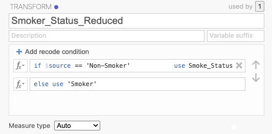

   

Table 22 Smoker status after recoding

Smoker_Status	Smoker_Status_Reduced
Non-smoker	Non-smoker
Occasional Smoker	Smoker
Regular Smoker	Smoker
Heavy Smoker	Smoker

Excluding Outliers (IQR method)

The IQR method flags values that lie more than 1.5 times the interquartile range above the third quartile or below the first quartile as outliers (more info).

The data below has two columns: Memory Score and its Absolute IQR value. The last two rows show extreme outliers (values of 15 and 98) with ABSIQR values above 1.5, indicating they fall outside the boxplot whiskers:

Table 23 Memory scores before filtering (ABSIQR)

Memory_Score	ABSIQR(Memory_Score)
68	0
66	0
70	0
…	…
15	9.05
98	5.05

To exclude these outliers:

1. Click the Data tab and select Filters.

2. Enter the expression: ABSIQR(Memory_Score) < 1.5

Table 24 Memory scores after filtering (ABSIQR)

Filter 1	Memory_Score	ABSIQR(Memory_Score)
✔	68	0
✔	66	0
✔	70	0
✔	…	…
✘	15	9.05
✘	98	5.05

The two outliers are excluded from all analyses and visualisations.

Excluding Outliers (z-score method)

The z-score method typically flags values with an absolute z-score greater than 3 as outliers, though stricter or more lenient thresholds can be applied.

Table 25 Memory scores before filtering (ABSZ)

Memory_Score	ABSZ(Memory_Score)
68	1.08
66	0.93
70	1.23
…	…
15	3.01
98	3.43

The last two rows show outlier values with absolute z-scores above 3. To exclude them:

1. Click the Data tab and select Filters.

2. Enter the expression: ABSZ(Memory_Score) < 3

Table 26 Memory scores after filtering (ABSZ)

Filter 1	Memory_Score	ABSZ(Memory_Score)
✔	68	1.08
✔	66	0.93
✔	70	1.23
✔	…	…
✘	15	3.01
✘	98	3.43

Restricting Analyses to a Subset of Data

To restrict all analyses to a single group, use a Filter. This is best when the excluded rows are of no interest at all.

Below is a dataset with Region, Education Level, and Total Survey Score. To analyse only participants from North America:

1. Click the Data tab and select Filters.

2. Enter the expression: Region == 'North America'

Table 27 Data before filtering

Region	Education Level	Total Survey Score
North America	High School	15
North America	University	20
Europe	High School	10
Europe	University	25

Table 28 Data after filtering to North America only

Filter 1	Region	Education Level	Total Survey Score
✔	North America	High School	15
✔	North America	University	20
✘	Europe	High School	10
✘	Europe	University	25

jamovi will include only the ticked rows in all subsequent analyses and visualisations.

Analysing Subsets of Data (Split File)

To analyse two or more subsets separately — equivalent to “Split File” in SPSS — the approach in jamovi requires creating a computed variable per subset using the FILTER() function.

Tip

This is a workaround for the absence of a native split-file feature. A more direct solution is planned for a future version of jamovi.

Using the same dataset as above, create one computed variable for each region:

1. Click a new column, choose New Computed Variable, name it Score_NorthAm, and enter:

   FILTER(`Total Survey Score`, Region == 'North America')

2. Repeat for Europe, naming it Score_Europe:

   FILTER(`Total Survey Score`, Region == 'Europe')

Table 29 Data after creating subset variables

Region	Education Level	Total Survey Score	Score_NorthAm	Score_Europe
North America	High School	15	15
North America	University	20	20
Europe	High School	10		10
Europe	University	25		25

Use Score_NorthAm and Score_Europe in separate analyses to compare Education Level effects within each region independently.

Attention Checks with a Reverse-Scored Item

Two items asking a similar question but worded in opposite directions can be used as an attention check. Participants who fail to respond consistently are likely not paying attention.

For example: - Item 1: “I never doubt my abilities.” - Item 2: “I often doubt my abilities.”

A participant who strongly agrees (5) with Item 1 should strongly disagree (1) with Item 2. First, reverse-score Item 2 (assuming a 1–5 scale):

Table 30 Step 1 — reverse score Item_2

Item_1	Item_2	Item_2_Reversed
5	1	5
1	5	1
1	2	4

Next:

1. Click a new column and choose New Computed Variable.

2. Compute the absolute difference between Item_1 and Item_2_Reversed:

   ABS(Item_1 - Item_2_Reversed)

Table 31 Step 2 — compute absolute difference

Item_1	Item_2	Item_2_Reversed	Abs_Difference
5	1	5	0
1	5	1	0
1	2	4	3

Finally:

1. Click the Data tab and select Filters.

2. Keep only participants with a difference of 0: Abs_Difference == 0

Table 32 Step 3 — filter out inconsistent respondents

Filter 1	Item_1	Item_2	Item_2_Reversed	Abs_Difference
✔	5	1	5	0
✔	1	5	1	0
✘	1	2	4	3

Only participants who responded consistently are included in analyses.

Attention Checks with a Single Item

A single attention check item instructs participants to select a specific response (e.g. “Please select ‘Strongly Agree’ for this item”). Any participant who selects a different response is likely not paying attention.

Below, Item_9 is an attention check instructing participants to select 5 on a 1–5 scale. Participant 3 selected 4 and should be excluded:

Table 33 Data before removing failed attention checks

ID	Item_1	Item_2	Item_9_Attention_Check
1	3	3	5
2	5	4	5
3	4	4	4

1. Click the Data tab and select Filters.

2. Enter the expression: Item_9_Attention_Check == 5

Table 34 Data after removing failed attention checks

Filter 1	ID	Item_1	Item_2	Item_9_Attention_Check
✔	1	3	3	5
✔	2	5	4	5
✘	3	4	4	4

Only participants who passed the attention check are included.

String Concatenation

String concatenation joins two or more text values into a single variable. This can be useful for combining categorical variables into a single grouping variable.

For example, combining Condition and Time into a single variable:

Table 35 Data before concatenation

Participant_ID	Condition	Time
1	Control	Pre
1	Control	Post
2	Therapy	Pre
2	Therapy	Post

1. Click a new column and choose New Computed Variable.

2. Name it Condition_Time and enter:

   Condition + '_' + Time

Table 36 Data after concatenation

Participant_ID	Condition	Time	Condition_Time
1	Control	Pre	Control_Pre
1	Control	Post	Control_Post
2	Therapy	Pre	Therapy_Pre
2	Therapy	Post	Therapy_Post

The underscore separator can be omitted or replaced with any other character.